


As the fog dissipated beneath the sea of trees it suddenly became all too clear that the fool had in fact been himself.
– safri
huh?
Lambda calculus is the back bone of functional programming, a type of programming that nobody can define.
So one way to define it is by a couple of characteristics:
- It’s based on the lambda calculus (huh?)
- Just a bunch of expressions innit
- expressions = values, variables, other functions
- Functions are first-class (like on airplanes)
- This literally just means that they can be put anywhere (including as an argument to another function)
Any language that is based solely on the lambda calculus is a pure functional programming language.
But apparently this is controversial, it can also refer to "referential transparency" where the
---
input -> function -> output
---
Where in other words, this is bad:
f(1) = X
f(2) = Y
Because they should get the same output
Fyi, this post probably isn’t useful to anybody.
Lambda Calculus
Recursive definition aside, the lambda calculus is a mathematical discovery that any program in existence can be created with three basic components:
- variables (a name for a value)
- abstractions (a function)
- expressions (variable, abstraction or both)
For the record, a “lambda” refers to the symbol “λ” but because I don’t know how to type that in emacs org-mode (what this blog is written in) example blocks so you get “\” instead.
The component we’ll spend most of our time looking at is abstractions.
Abstractions
Abstractions consist of two parts:
- da head
- da body
Take this dead simple lambda abstraction right here:
\x.x
- head < everything including and to the left of the period, lambda + variable + separator
- body > everything right of the period (the expression)
If you wanted a peak at Lambda Calculus 102, a more advanced function could look like:
(\x.x+1)
---
NOTE: I don't know how to input lambda's in emacs org-mode (how I write this blog) example codeblocks so just think of the lambda symbol when you see "/"
Now if you look even closer you might notice that there’s two x’s
This is a subtle hint to the fact that the x is in our head is the functions parameter where all x’s in the
Upon evaluation, this function is passed an input, to which that input then substitutes all x’s in the body
(\x.x+1) 4 = 5 :D
Alpha Equivalence
The author of Haskell Programming From First Principles really liked fancy words so I’m sorry but I shalst continue that trend here.
Alpha Equivalence basically just says that the letter we set as x has no meaning, value and is worthless.
\x.x
\y.y
\z.z
All represent the same function (😱)
Beta Reduction
Broadly speaking, beta reduction is the process where you substitute what you know about a function using a given input.
(\x.x) 5 = 5
This seems really simple until you start adding more abstractions:
(\x.x)(\y.y)
Here’s the definition I got for that:
In this case, we’d substitute the entire abstraction in for x. We’ll use a new syntax here, [x := z], to indicate that z will be substituted for all occurrences of x (here z is the function λ y.y).
Huh?
But it makes slightly more sense after applying the argument z and with this reduction:
((\x.x)(\y.y))z
  [x := (\y.y)]
           (\y.y)z
           [y := z]
                    z
But I’ve given up on understanding what in the hell they mean by “[x := z]”.
Our understanding goes as such:
Whenever you see [ x := y ], the right side substitutes the variable in the left side
ONWARD!!
Free Variables
B-b-b-but what happens if you add a variable that’s not in the abstraction’s head??
That would be a “free variable” which describes variables not defined in the head.
\x.xy
--- The free variable is y
CURRYYYYYY!!!!
One really fun feature of lambda calculus is that functions can quite literally only take one argument.
Something like:
\xy.xy
Is actually not possible in lambda calculus but the handsome Haskell Curry decided to make it possible anyways
The rule itself remains true, the above is just two nested lambdas:
\x.(\y.xy)
Where applying say “3” would reduce down to:
(\y.3 y)
But only actual masochists would enjoy writing that so functional programming languages usually make a secret handshake with the syntactic sugar kingdom and pretend that functions can take two arguments.
This becomes relatively clear with an example:
\xy.x + y
(\xy.x + y) 1 2
(\x.(\y.x + y)) 1 2
[x := 1]   --- replace the x with 1 :p
(\y. 1 + y) 2
[y := 2]   --- :p
1 + 2
3
:D
In this final state we’ve achieved something called beta normal form which is a fancy of way of saying it can’t be simplified further
In programming, beta normal form refers to the complete evaluation of a program!
This means that functional programming is literally just reducing functions with information that we know.
K that’s all fine but let’s get a bit more complicated:
(\xyz.xz(yz))(\mn.m)(\p.p)
This gets really hard to explain with text so here’s a break down of the process color coded by abstraction.
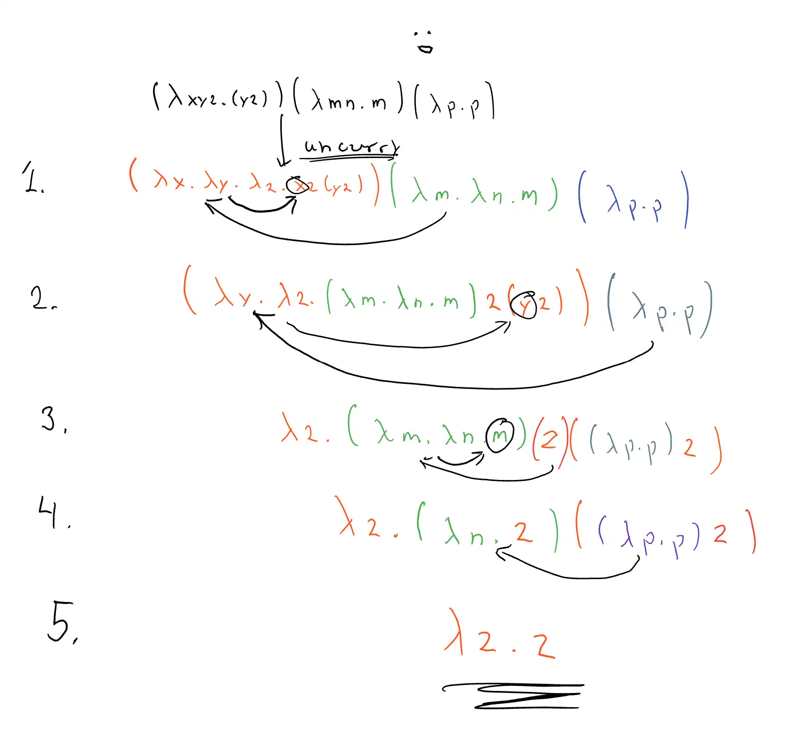
You’ll notice how at the end there we were able to discard the entirety of:
((\p.p)z)
As it was meant to replace all of the n’s in
(\n.z)
But there were no n’s!! Leaving us just with z
Combinators
Combinators are abstractions with no free variables,
It just combines the arguments given innit
These are combinators:
\x.x
\xyz.xyz
I feel like this isn’t a very useful word but I digress.
Divergence
It’s important to take this time to acknowledge the fact that some not so good functions choose not to reach their true beta normal form.
Normally, an abstraction will reduce into a nice neat little form but happens when the reduction creates a loop?
(\x.xx)(\x.xx)
The second abstraction is taken as an input to the first, replacing all instances of “x”, with that we get:
(\x.xx)(\x.xx)
Oh yea huh that’s a problem.
Abstractions of this nature “diverge” rather than “converge” and thus will never reduce to a beta normal form.
I thought this was a programming blog
Oh yea oops.
What’s really interesting about lambda calculus and functional programming is that all code execution is beta reduction.
If we take the haskell code:
ghci> (\x -> x*x) 3
9
We can see that it’s damn near exactly the same syntax we’ve been looking at.
The reduction follows the order:
- Oh hey I’m replacing all of my x’s with ‘3’
- K now I’m multiplying x by itself
- (outputs)
In another example, we can take simple arithmetic:
100 / 2In this case our function is literally the division operator “/”, we can reduce it by simply evaluating the expression:
50Credit
Tbh I don’t really have a target audience for this post as anybody that would willingly click on a post about lambda calculus is probably smarter than me anyways.
I didn’t really add any special knowledge either, I just read the first chapter of Haskell Progrmaming From First Principles (which you can read a sample of here) and watched the video Programming with Math | The Lambda Calculus made by the YouTuber Eyesomorphic.
So you should just use those tbh.